Deep Learning for Solving and Estimating Macroeconomic Models
WGEM, Frankfurt am Main
ECB
2026-06-30
Motivation
- Quantitative macro models can be:
- Nonlinear (occasionally binding constraints, large shocks)
- High-dimensional (many state variables, distributions in HANK)
- Richly parameterized
- Classical solution methods:
- Rely on local linearization, low-order perturbation, grids …
- Infeasible to globally solve nonlinear high dimensional models
This Limits
- The class of models we can solve globally
- The models we can estimate with full-information likelihood methods
How to use deep learning to overcome these hurdles
- Following Kase, Melosi, Rottner (2025) “Estimating Nonlinear Heterogeneous Agent Models with Neural Networks”
- Practical code example for a simple three-equation New-Keynesian model
Method at a glance
1. Extended Neural Network
- Use a deep neural network to approximate the policy function
- Treat parameters as pseudo-state variables
Avoids repeatedly solving the model
- Deep neural networks are great at approximating high dimensional functions
2. Neural Network Particle Filter
- Evaluating the likelihood of a complex model can be costly
- Particle filter becomes the bottleneck for estimation
Reduces the cost of likelihood evaluations
- Use the particle filter to generate a dataset of parameters and likelihoods
- Fit a deep neural network on it - create a surrogate model for the particle filter
Solving the model with deep neural networks
Euler residual minimization (following Maliar et al. 2021)
Replace continuum of agents by a finite but large number \(L\) of agents
Parameterize individual and aggregate policy functions with deep NNs:
\[ \psi_t^i = \psi^{I}_{NN}(S_t^i, S_t \mid \Theta), \qquad \psi_t^A = \psi^{A}_{NN}(S_t \mid \Theta) \]
\(S_t = \{\{S_t^i\}_{i=1}^L, S_t^A\}\) – state vector and \(\Theta\) – structural parameters of the model
- Construct a loss function:
- Weighted mean of squared Euler / equilibrium residuals
- Train the neural networks using stochastic optimization:
- Minimize the loss for points drawn from the state space
- Simulate the model forward to generate new points in the state space
Bottleneck for estimation
Training these networks from scratch for each parameter vector \(\Theta\) would be far too costly inside a likelihood-based estimation routine
Extended Neural Network
💡 Treat parameters as pseudo states
Again, work with a finite but large number \(L\) of agents instead of a continuum
Parameterize individual and aggregate policy functions with extended deep NNs:
\[ \psi_t^i = \psi^{I}_{NN}(S_t^i, S_t, \textcolor{orange}{\tilde{\Theta_{}}} \mid \bar{\Theta_{}}), \qquad \psi_t^A = \psi^{A}_{NN}(S_t, \textcolor{orange}{\tilde{\Theta_{}}} \mid \bar{\Theta_{}}) \]
\(S_t = \{\{S_t^i\}_{i=1}^L, S_t^A\}\) – state vector, \(\bar{\Theta_{}}\) – fixed parameters, \(\tilde{\Theta_{}}\) – parameters to estimate
Construct a loss function, as before
Train the extended NNs using stochastic optimization:
- Minimize the loss for points drawn from the state space
- Draw new values for parameters \(\tilde{\Theta_{}}\)
- Simulate the model forward to generate new points in the state space
More complex problem, but still feasible and we can amortize the cost
- We train the extended networks only once and can evaluate the model for different parameter values without re-solving it
Practical example 🛠️ – solving a simple model
Small linearized DSGE model
- Small linearized three-equation New-Keynesian model with a TFP shock
\[ \begin{aligned} \hat{X}_t &= E_t \hat{X}_{t+1} - \sigma^{-1}\Bigl(\phi_{\Pi}\hat{\Pi}_t + \phi_Y \hat{X}_{t} - E_t \hat{\Pi}_{t+1} - \hat{R}_t^{\ast}\Bigr) \\ \hat{\Pi}_t &= \kappa \hat{X}_t + \beta E_t \hat{\Pi}_{t+1} \\ \hat{R}_t^{\ast} &= \rho_A \hat{R}_{t-1}^{\ast} + \sigma (\rho_A-1)\omega\sigma_A\epsilon_t^A \end{aligned} \]
Where, \(\hat{X}_t\) – output gap, \(\hat{\Pi}_t\) – inflation, \(\hat{R}_t^\ast\) – natural rate of interest
- Analytical solution to the model to check against
\[ \begin{aligned} \hat{X}_t &= \frac{1 - \beta \rho_A} {(\sigma(1-\rho_A) + \phi_Y)(1-\beta\rho_A) + \kappa(\phi_\Pi - \rho_A)} \, \hat{R}_t^{\ast} \\ \hat{\Pi}_t &= \frac{\kappa} {(\sigma(1-\rho_A) + \phi_Y)(1-\beta\rho_A) + \kappa(\phi_\Pi - \rho_A)} \, \hat{R}_t^{\ast} \end{aligned} \]
General setup
You can find the notebook on GitHub in the examples folder (analytical.ipynb):
https://github.com/tseep/estimating-hank-nn
- We use
pytorchas the backbone deep learning framework
- The model is defined in the
NKModelclass, with the methods that:- create a suitable neural network (
make_network) - define the economic model (
policy,residuals,steady_state) - initialize the model (
initialize_state) - draw shocks or parameters (
draw_shocks,draw_parameters) - simulate the model (
step,steps,sim_step,simulate) - train the neural networks (
loss,train_model)
- create a suitable neural network (
In short:
- To create the model object:
# Parameters
NK_par = {
    "beta": 0.97,
    "sigma": 2.0,
    "eta": 1.125,
    "phi": 0.7,
    "phipi": 1.875,
    "phiy": 0.25,
    "rho_a": 0.875,
    "sigma_a": 0.06,
}

# Ranges for parameters
NK_range = {
    "beta": torch.distributions.Uniform(0.95, 0.99),
    "sigma": torch.distributions.Uniform(1.0, 3.0),
    "eta": torch.distributions.Uniform(0.25, 2.0),
    "phi": torch.distributions.Uniform(0.5, 0.9),
    "phipi": torch.distributions.Uniform(1.25, 2.5),
    "phiy": torch.distributions.Uniform(0.0, 0.5),
    "rho_a": torch.distributions.Uniform(0.8, 0.95),
    "sigma_a": torch.distributions.Uniform(0.02, 0.1),
}

# Distribution for the shock process innovations
shock_dist = {
    "zeta": torch.distributions.Normal(0.0, 1.0),
}

# Create the model object
model = NKModel(NK_par, NK_range, shock_dist)- To solve the model
Easy peasy lemon squeezy 🍋
Step 1. Parametrize with NNs
We approximate the unknown control variables, \(\hat{X}_t\) and \(\hat{\Pi}_t\), with a deep neural network:
\[ \begin{pmatrix} \hat{X}_t \\ \hat{\Pi}_t \end{pmatrix} = \psi\bigl(S_t,\tilde{\Theta}\mid\bar{\Theta}\bigr) ≈ \psi_{\mathrm{NN}}\bigl(\hat{R}_t^{\ast},\;\beta,\;\sigma,\;\eta,\;\varphi,\;\phi_{\Pi},\;\phi_{Y},\;\rho_{A},\;\sigma_{A}\bigr) \]
- Create a neural network
def make_network(
    self,
    N_states=1,
    N_par=None,
    N_outputs=2,
    hidden=64,
    layers=5,
    activation=torch.nn.CELU(),
    normalize=True,
):
    # Detect device
    device = self.par.values()[0].device

    # Number of parameters
    if N_par is None:
        N_par = len(self.par)
    N_inputs = N_states + N_par

    layer_list = []

    # Normalize layer
    if normalize:
        lb = torch.cat([-torch.ones(N_states, device=device), self.range.low_tensor()], dim=-1)
        ub = torch.cat([+torch.ones(N_states, device=device), self.range.high_tensor()], dim=-1)
        layer_list.append(NormalizeLayer(lb, ub))

    # First layer
    layer_list.append(torch.nn.Linear(N_inputs, hidden))
    layer_list.append(activation)

    # Middle layers
    for _ in range(1, layers):
        layer_list.append(torch.nn.Linear(hidden, hidden))
        layer_list.append(activation)

    # Last layer
    layer_list.append(torch.nn.Linear(hidden, N_outputs))

return torch.nn.Sequential(*layer_list)- Feed inputs to the neural network and process outputs
def policy(self, state=None, par=None):
        if state is None:
            state = self.state
        if par is None:
            par = self.par_draw

        # Vector of states and parameters
        input_state = state.cat()
        input_par = par.cat()

        # Expand if necessary (for calculating expectations)
        if input_state.ndim > input_par.ndim:
            input_par_shape = list(input_par.shape)
            input_par_shape.insert(0, input_state.size(0))
            input_par = input_par.unsqueeze(0).expand(input_par_shape)

        # Prepare the input by concatenating states and parameters
        input = torch.cat([input_state, input_par], dim=-1)

        # Evaluate the network
        output = self.network(input)

        # Assign and scale the output
        X = output[..., 0:1] / 100
        Pi = output[..., 1:2] / 100

        return X, Pi
Step 2. Construct residuals and loss function
- Objective is to find NN weights so that residuals for equilibrium conditions are close to zero
\[ \begin{aligned} &\text{ERR}^{\,i}_{\text{IS}} = \hat{X}_t^i - E_t \hat{X}_{t+1}^i - \sigma^{-1} \bigl( \phi_\Pi \hat{\Pi}_t^i + \phi_Y \hat{X}_t^i - E_t \hat{\Pi}_{t+1}^i - \hat{R}_t^{\ast\,i} \bigr) \\ &\text{ERR}^{\,i}_{\text{NKPC}} = \hat{\Pi}_t^i - \kappa \hat{X}_t^i - \beta E_t \hat{\Pi}_{t+1}^i \end{aligned} \]
def residuals(self, e):
    par = self.par_draw
    ss = self.ss
    state = self.state

    # Output gap and inflation period t
    X, Pi = self.policy(self.state, self.par_draw)

    # Next period state
    state_next = self.step(e)

    # Expected output gap and inflation period t+1
    X_next, Pi_next = self.policy(state_next, self.par_draw)
    EX_next = torch.mean(X_next, dim=0)
    EPi_next = torch.mean(Pi_next, dim=0)

    # Residuals
    ERR_NKPC = Pi - (ss.kappa * X + par.beta * EPi_next)
    ERR_IS = X - (EX_next - 1 / par.sigma * (par.phipi * Pi + par.phiy * X - EPi_next - state.zeta))

return ERR_NKPC, ERR_IS- Combine the residuals into a scalar loss
\[ \mathcal{L} = w_1 \cdot \frac{1}{B} \sum_{i=1}^{B} \left( \text{ERR}^{\,i}_{\text{IS}} \right)^2 + w_2 \cdot \frac{1}{B} \sum_{i=1}^{B} \left( \text{ERR}^{\,i}_{\text{NKPC}} \right)^2 \]
Step 3. Training to minimize the loss
- We simulate the economy and minimize the loss, drawing new parameters from time to time, …
def train_model(
    self,
    iteration=10000,
    internal=5,
    steps=10,
    batch=100,
    mc=10,
    par_draw_after=1,
    lr=1e-3,
    eta_min=1e-10,
    device="cpu",
    print_after=100,
):
    # Save training configuration
    self.training_conf = locals().copy()

    # Print training configuration
    print("Training configuration:")
    for key, value in self.training_conf.items():
        if key != "self":
            print(f"{key}: {value}")

    # Set the network to train mode
    self.network.train()
    self.network.to(device)

    # Initialize
    self.par_draw = self.draw_parameters(shape=(batch, 1), device=device)
    self.state = self.initialize_state(batch=batch, device=device)
    self.ss = self.steady_state()

    # Starting weights for loss components
    weights = [1.0, 1.0]

    # Optimizer and scheduler
    optimizer = torch.optim.AdamW(self.network.parameters(), lr=lr)
    scheduler = torch.optim.lr_scheduler.CosineAnnealingLR(optimizer, T_max=iteration, eta_min=eta_min)

    # Dictionary for loss
    self.loss_dict = {"iteration": [], "total": [], "nkpc": [], "is": []}

    # Progress bar
    pbar = trange(iteration)

    # Training loop
    running_loss = 0.0
    for i in pbar:
        for o in range(internal):
            optimizer.zero_grad()
            e = self.draw_shocks((mc, batch, 1), antithetic=True, device=device)
            nkpc, bond_euler = self.residuals(e)
            loss, loss_components = self.loss(nkpc, bond_euler, batch=batch, weights=weights)
            loss.backward()
            torch.nn.utils.clip_grad_norm_(self.network.parameters(), 1.0)
            optimizer.step()

            # Record loss
            if o == 0:
                self.loss_dict["iteration"].append(i)
                self.loss_dict["total"].append(loss.item())
                for key, value in loss_components.items():
                    self.loss_dict[key].append(value.item())

                # Running loss
                running_loss += loss.item() / batch

        # Print running loss in the progress bar after 100 iterations
        if i % print_after == 0:
            pbar.set_postfix(
                {
                    "lr:": scheduler.get_last_lr()[0],
                    "loss": running_loss / print_after,
                }
            )
            running_loss = 0.0

        # Update learning rate
        scheduler.step()

        # Draw new parameters
        if i % par_draw_after == 0:
            self.par_draw = self.draw_parameters((batch, 1), device=device)
            self.ss = self.steady_state()

        # Sample states by simulation
        self.steps(batch=batch, device=device, steps=steps)

    # Set network to evaluation mode
    self.network.eval()
Let’s check the loss

Let’s check the loss components

What happened during training

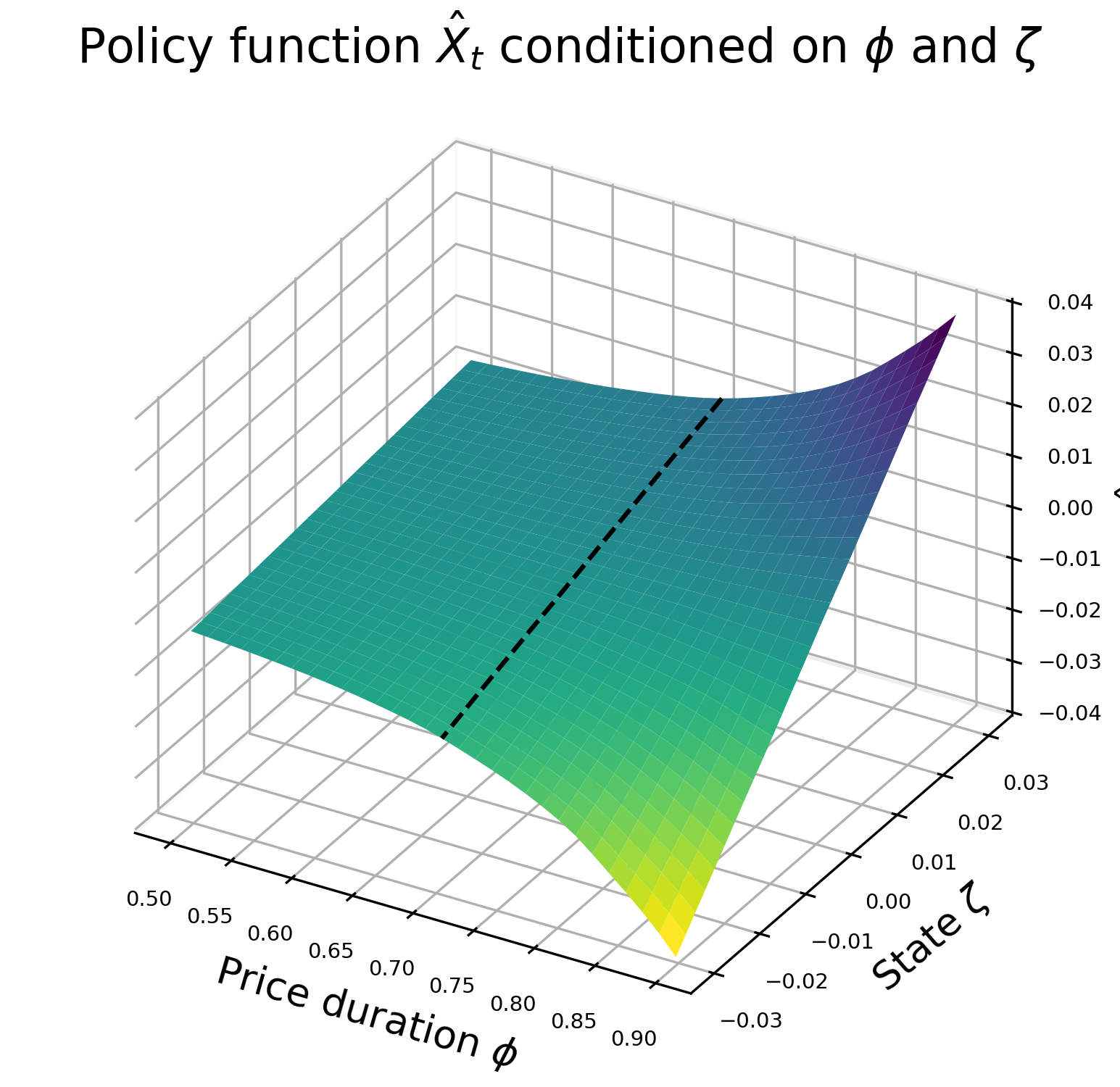
Neural network solution over states and parameters
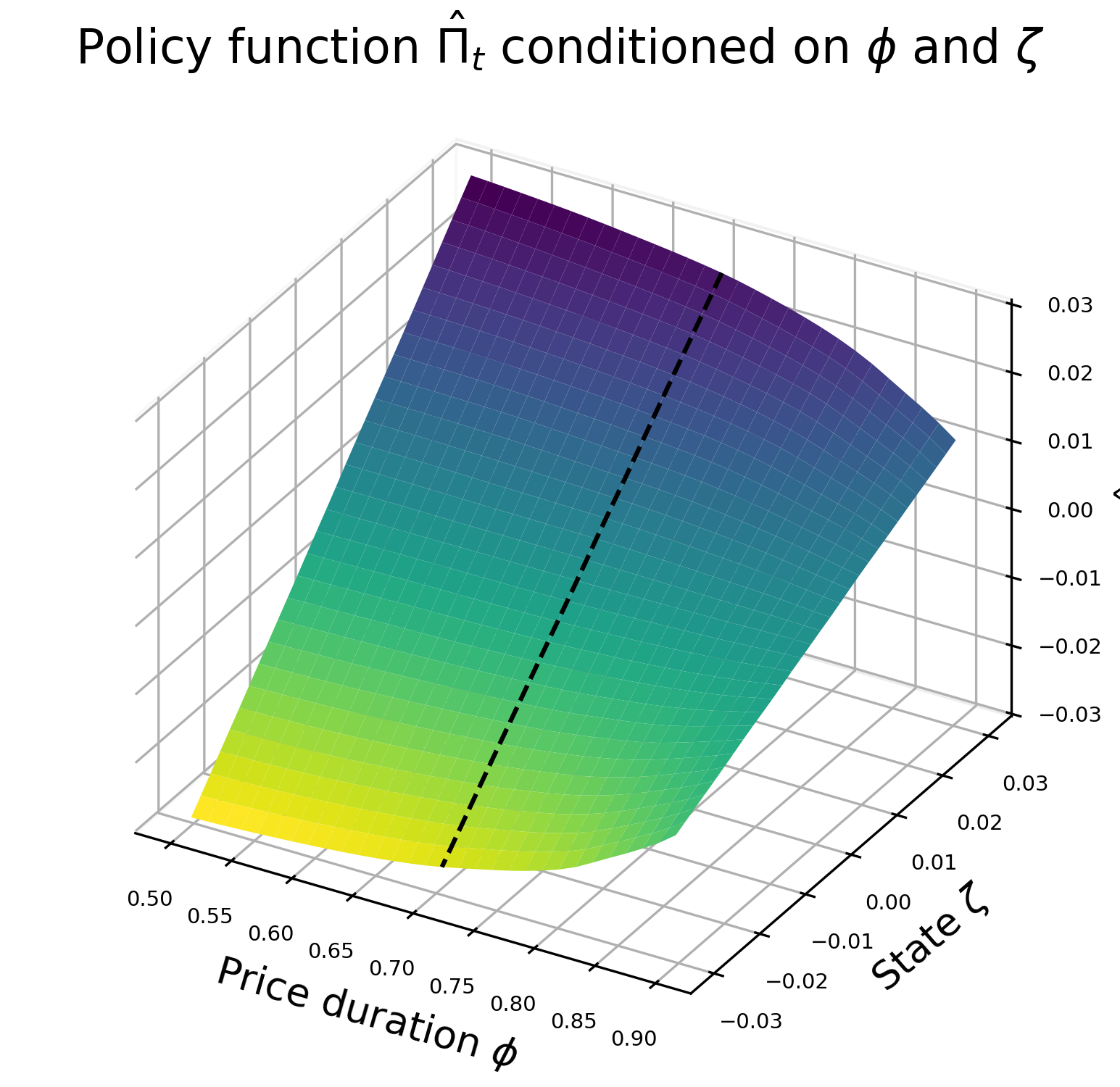
Compared to the analytical solution - \(\hat{\Pi_t}\)

Compared to the analytical solution - \(\hat{X_t}\)

Practical example 🛠️ – estimating a simple model
Deep learning for estimation
Evaluating the likelihood with a particle filter is slow
The particle filter becomes a bottleneck for estimation
Neural Network Particle Filter – Train a neural network to approximate:
\[ \Theta \;\mapsto\; \log \mathcal{L}(\Theta) \]
Training procedure
- Generate dataset of parameter draws and log-likelihoods
- Split into training and validation sets
- Train a NN on the training set
- Use validation set to control for overfitting
Benefits
- ⚡ Single likelihood evaluation becomes almost instantaneous
- 🔇 Smooths out noise from filtering
- 🔁 Enables efficient Bayesian estimation
Estimation on simulated data
- Simulate some data
- Compute the covariance matrix \(R\) and add measurement error
Neural Network Particle Filter
- Create a dataset of parameter values and likelihoods
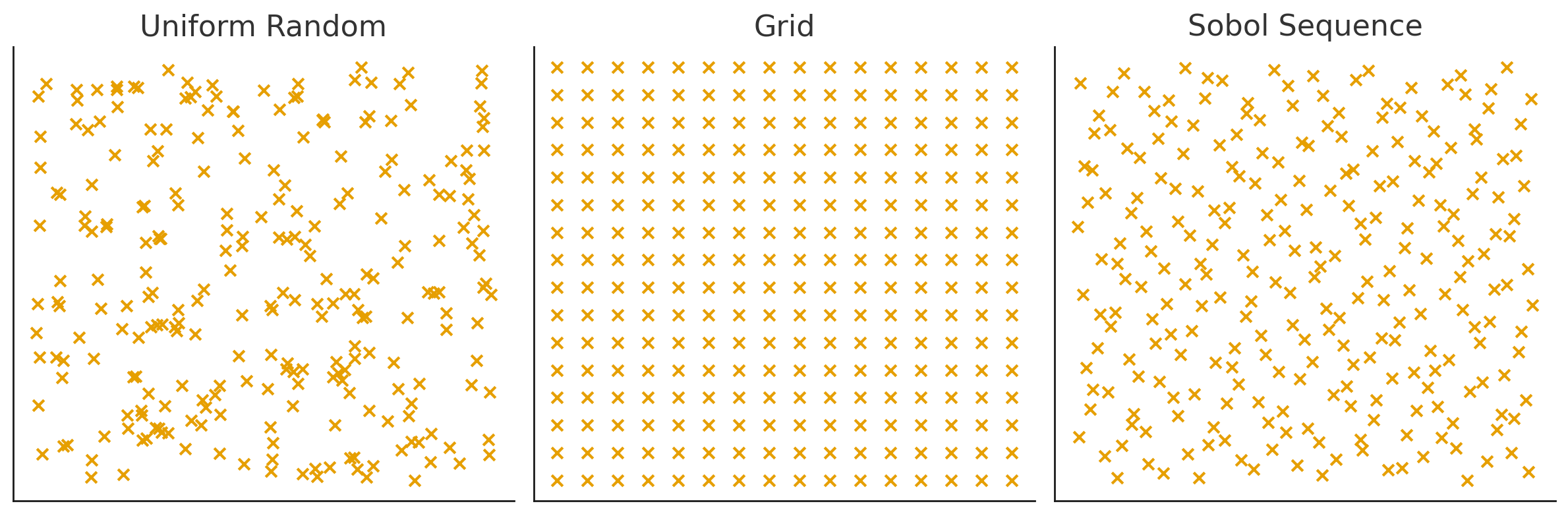
2. Create a dataset of parameter values and likelihoods
Using Sobol sequence to cover the parameter space more efficiently.
def filter_dataset(
    self,
    par_names=None,
    N=1000,
    par=None,
    P=1000,
    sim=100,
    device="cpu",
    sobol=False,
):
    # Make a copy of par
    if par is None:
        par = deepcopy(self.model.par)

    # Parameters that vary in the dataset
    if par_names is None:
        par_names = par.keys()

    # Create Sobol draws if necessary
    if sobol:
        sampler = torch.quasirandom.SobolEngine(
            len(par_names),
        )
        sobol_draws = sampler.draw(N).squeeze(-2)

    par_list = []
    log_likelihood_list = []
    for n in trange(N):
        # Draw parameters
        par_draw = {}
        idx = 0
        for key in par.keys():
            if key in par_names:
                if sobol:
                    low = self.model.range.get(key).support.lower_bound
                    high = self.model.range.get(key).support.upper_bound
                    par_draw[key] = low + (high - low) * sobol_draws[n, idx].view(1)
                    idx += 1
                else:
                    par_draw[key] = self.model.range.get(key).sample((1,))
            else:
                par_draw[key] = par.get(key)

        # Convert to Parameters object
        par_draw = Parameters(par_draw)

        # Calculate likelihood
        log_likelihood, _ = self.filter(P, par=par_draw, sim=sim, device=device)

        # Store
        par_list.append(par_draw.cat())
        log_likelihood_list.append(log_likelihood)

    # Create dataset by stacking par_list together and log_likelihood_list together
    par_tensor = torch.stack(par_list, dim=0)
    log_likelihood_tensor = torch.stack(log_likelihood_list, dim=0)

    self.dataset = {"par": par_tensor, "log_likelihood": log_likelihood_tensor}
4. Train the neural network
Note that this is supervised training. We have the whole dataset ready and can efficiently process it by creating a DataLoader.
def train(
    self,
    batch=64,
    epochs=10000,
    device="cpu",
    lr=1e-3,
    eta_min=1e-6,
    validation_share=0.2,
    print_after=1000,
):
    # Create optimizer and scheduler
    optimizer = torch.optim.AdamW(self.network.parameters(), lr=lr)
    scheduler = torch.optim.lr_scheduler.CosineAnnealingLR(optimizer, T_max=epochs, eta_min=eta_min)

    # Randomly shuffle the dataset
    idx = torch.randperm(self.dataset["par"].size(0))
    self.dataset["par"] = self.dataset["par"][idx, ...]
    self.dataset["log_likelihood"] = self.dataset["log_likelihood"][idx, ...]

    # Split dataset into training and validation samples
    N = self.dataset["par"].size(0)
    N_train = int(N * (1 - validation_share))
    dataset_train = torch.utils.data.TensorDataset(
        self.dataset["par"][:N_train, ...],
        self.dataset["log_likelihood"][:N_train, ...].unsqueeze(-1),
    )
    dataset_validation = torch.utils.data.TensorDataset(
        self.dataset["par"][N_train:, ...],
        self.dataset["log_likelihood"][N_train:, ...].unsqueeze(-1),
    )

    # Create dataloader for training and validation
    dataloader_train = torch.utils.data.DataLoader(dataset_train, batch_size=batch, shuffle=True)
    dataloader_validation = torch.utils.data.DataLoader(dataset_validation, batch_size=batch, shuffle=True)

    # Set the network to train mode
    self.network.train()
    self.network.to(device)

    # Progress bar
    pbar = trange(epochs)

    # Dictionary for loss
    self.loss_dict = {"iteration": [], "training_loss": [], "validation_loss": []}

    # Training loop over epochs
    for i in pbar:
        for x, y in dataloader_train:
            # Move to device
            x = x.to(device)
            y = y.to(device)

            # Forward pass
            y_hat = self.network(x)

            # Loss
            loss = torch.nn.functional.mse_loss(y_hat, y)

            # Backward pass
            optimizer.zero_grad()
            loss.backward()
            # torch.nn.utils.clip_grad_norm_(self.network.parameters(), 1.0)
            optimizer.step()

        # Update learning rate
        scheduler.step()

        # Print training and validation loss in the progress bar after x epochs
        if i % print_after == 0:
            # Training loss
            with torch.no_grad():
                training_loss = 0.0
                for x, y in dataloader_train:
                    x = x.to(device)
                    y = y.to(device)
                    y_hat = self.network(x)
                    training_loss += torch.nn.functional.mse_loss(y_hat, y, reduction="sum").item()
                training_loss = training_loss / len(dataset_train)

            # Validation loss
            with torch.no_grad():
                validation_loss = 0.0
                for x, y in dataloader_validation:
                    x = x.to(device)
                    y = y.to(device)
                    y_hat = self.network(x)
                    validation_loss += torch.nn.functional.mse_loss(y_hat, y, reduction="sum").item()
                validation_loss = validation_loss / len(dataset_validation)

            # Record training and validation loss in the dictionary
            self.loss_dict["iteration"].append(i)
            self.loss_dict["training_loss"].append(training_loss)
            self.loss_dict["validation_loss"].append(validation_loss)

            # Update progress bar
            pbar.set_postfix(
                {
                    "lr:": scheduler.get_last_lr()[0],
                    "training": training_loss,
                    "validation": validation_loss,
                }
            )

    # Set network to evaluation mode
    self.network.eval()
Let’s check the training and validation losses

Cut through the noise 🎧

Recovering the truth 🔎

Thank you! 🙏
You can find the Jupyter notebook here!
https://github.com/tseep/estimating-hank-nn
